Questions:

1

2

3

4

5

6

7

8

9

10

11

12

13

14

15

16

17

18

19

20

21

22

23

24

25

26

Electrostatic Potential Solutions

Potential difference

1. (a) E = 5x²i. Calculate ΔV between x = 0 m and x = 4 m.

(b) E = (2/y)j. Calculate ΔV between y = 2 m and y = 5 m.

The potential difference between two points is defined as

ΔV = −∫_i^fE · dl ,

where dl is the parallel to the path of integration. The potential difference is independent of the path taken, so one may choose whichever path makes the integration easiest.

(i) We will integrate along the line joining the two points so that dl = idx.

ΔV	= −∫ifE · dl
	= −∫04 5x2i · i dx
	= −∫04 5x2dx
	= −(5/3) x3 |04
	= −320/3 Volts

Therefore V(x=4) is at a lower potential than V(x=0).

(b) We will integrate along the line joining the two points so that dl = jdy.

ΔV	= −∫ifE · dl
	= −∫25 (2/y) j · j dy
	= −∫25 2dy / y
	= −2 ln(y) |25
	= −2 ln(5/2) Volts

Therefore V(y=5) is at a lower potential than V(y=2).



---



2. The electric field between the plates of a capacitor is 1000 V/m and zero everywhere else. The plates are 1.0 mm apart. Put the origin at the positive plate and have the negative plate at x = 1.0 mm. What is the potential difference between x = 0.25 mm and x = 0.75 mm. Which point has the higher potential?

   First let's sketch the field and note the area we are looking for

   

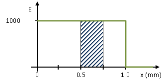
   The potential difference between two points is defined as

                ΔV = V(A) – V(B) = –∫_i^f E•dl ,

   where dl is the parallel to the path of integration. Since the electric field coordinate system has x lying in the i direction, and since we are moving out in the same direction, E•dl = E i•idx = Edx.

   ΔV	= –∫if E•dl
   V(.75)  – V(.25)	= –∫0.250.75 Edx
   	= – ∫0.250.75 (1000 V/m) dx
   	= –(1000 V/m) x |0.250.75
   	= –(1000 V/m) (0.50 mm)
   	= –0.50 V

   Note that the potential difference is just the negative of the area under the E versus x graph. Finding that area is very simple in this case, ΔV = – 1000 V/m  × (0.75 – 0.50) mm = –0.50 V.

   Since the electric field is positive to the right, the positive charge is at the origin so x = 0.25 mm is at higher potential.



---

3. An electric field is given in the diagram below.

   (a) What is V(b) – V(a)?
   

   (b) What is V(b) – V(c)?
   

   (c) Find point(s) d so that the V(d) – V(c) = +50.0 Volts.
   

   
   
   
   
   Note on the graph that each small block has an area of 25 Volts.
   

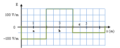
   (a)    We want the negative of the area from a (1 m) to b (3m). From the graph this is +2 blocks or –50 Volts.  Since V(b) = V(a) – 50 V, V(b) is at lower potential.
   
   

   (b)    We want the negative of the area from c (4.5 m) to b (3m). Since we are moving backwards, this is equivalent to the positive area from 3 m to 4.5 m, +5 blocks or +125 Volts.  Since V(b) = V(c) + 125 V, V(b) is at higher potential.
   
   

   (c)    If point d is to the right of point c, then we want a negative area of the curve equal to 50 Volts (2 blocks) since the voltage difference is the negative of that value. That occurs at d = 5.5 m.
   
   If point d is to the left of point c, we are going backwards and thus we want a positive area of the curve from d to c equal to 50 Volts (2 blocks). That occurs at d = 3.5 m.
   

   

   ---
4. Find the electrostatic potential difference between points A and B which are distances r_A = 1.0 m and r_B = 2.0 m from an infinitely long thin wire with λ = 1.0 μC/m. The result E = λ/2πε₀r is useful. If an electron (q = −e = −1.602 × 10⁻¹⁹ C and mass m_e = 9.11 × 10⁻³¹ kg) is released from rest at point B, what is it's speed at point A?



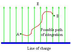
We are given that the electric field is

E = E(r)r = (λ/2πε₀r)r ,

where r is the unit radial vector pointing outward from the wire.

The potential difference between two points is defined as

ΔV = V(A) − V(B) = −∫_A^BE · dl ,

where dl is the parallel to the path of integration. Since the electric field is radial, the dot product picks out portion of dl which is parallel to r.

V	= −∫ABE · dl
	= −∫AB E dr
	= −(λ/2πε0) ∫12 dr/r
	= −(2kλ) ln(r) |12
	= −(2kλ) ln(2)
	= −2(8.99 × 109 N−m2/C2)(1 × 10−6 C/m) ln(2)
	= −1.2463 × 104 Volts

The minus sign indicates that point V(B) is smaller than V(A) or that point B at a lower potential than point A (i.e. farther from the positive charge). Therefore a negative particle released from rest at point B will accelerate towards point A (high potential). Using conservation of energy

½m(v_A)² − ½m(v_B)²  = qΔV .

Since v_B = 0, solving for v_A yields

vA	= [2qV/m]½
	= [2(−1.602 × 10−19 C)(−1.2463 × 104 V)/(9.11 × 10−31 kg)]½
	= 6.6 × 107 m/s

The charge will be moving at 6.6 × 10⁷ m/s when it reaches point A.



---

5. Find the electrostatic potential between points A and B which are distances x_A = 1.0 m and x_B = 2.0 m from an infinitely large thin plate with σ = 1.0 μC/m². The result E = σ/2ε₀ is useful. If an electron (q = −e = −1.602 × 10⁻¹⁹ C and mass m_e = 9.11 × 10⁻³¹ kg) is released from rest at point A, what is it's speed at point B?.



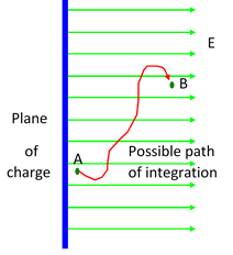
We are given that the electric field is

E = E i = (σ/2ε₀)i ,

where i is the unit vector pointing outward from the plane.

The potential difference between two points is defined as

ΔV = V(A) − V(B) = −∫_i^fE · dl ,

where dl is the parallel to the path of integration. Since the electric field only has an i component, the dot product picks out portion of dl which is parallel to i.

V	= −∫ifE · dl
	= −∫AB E dx
	= −(σ/2ε0) ∫12 dx
	= −(2kσ) x |12
	= −2kσ
	= −2(8.99 × 109 N−m2/C2)(1 × 10−6 C/m2)
	= −5.6486 × 104 Volts

The minus sign indicates that point A is at a lower potential than point B. Therefore a negative particle released from rest at point A will accelerate towards point B. Using conservation of energy

½m(v_B)² − ½m(v_a)² = qΔV .

Since v_B = 0, solving for v_A yields

vA	= [2qV/m]½
	= [2(−1.602 × 10−19 C)(−5.6486 × 104 V)/(9.11 × 10−31 kg)]½
	= 1.4 × 108 m/s

If started from rest, an electron will be moving at 1.4 × 10⁸ m/s when it reaches point A. This is almost half the speed of light!



---

6. The electric field due to a large plate is E = σ/2ε₀ as we have seen. A capacitor consists of two identical plates with equal but opposite charge distributions.

(a) Show that the net electric field is zero outside the plates and E_net = σ/ε₀ between the plates.
(b) Show that the potential difference between the plates is directly proportional to the separation d of the plates.

(a) Let's first sketch the field due to each plate. The electric field for the positive plate is shown by the dashed red lines leaving the plate. The electric field for the negative plate is shown by the solid green red lines entering the plate.



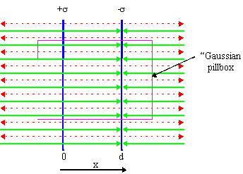
As can be seen, there are an equal number of solid and dashed lines. Outside the plates, the dashed and solid lines are anti−parallel and thus cancel. Between the plates, both sets of lines point in the same direction and thus add. To be more formal, we can make use of Gauss' Law,

∫E · ndA = Q_enclosed/ε₀ ,

where n is the outward−looking normal on each side of the surface. The pillbox has two ends and one side, so that the integral has three parts

∫E · ndA = ∫_leftE · n_left dA + ∫_sideE · n_sidedA + ∫_rightE · n_rightdA .

By symmetry the field on either side is horizontal, with no lines crossing the sides of the "gaussian pillbox". Thus E · n_side = 0 and the integral for the side of the pillbox vanishes. Symmetry also demands that if the electric field is not zero it must be equal and opposite on either side of the capacitor. Thus E · n_left = E · n_right = E_outside. Hence the integrals reduce to

∫_leftE · n_left dA + ∫_sideE · n_sidedA + ∫_rightE · n_rightdA = 2E_outside∫dA .

The integral over the area is just the area of the end of the pillbox, A. So Gauss's law is

2E_outsideA = Q_enclosed/ε₀ .

Since the plate have equal and opposite charges, we know Q_enclosed = 0. Hence E_outside = 0 as we would expect from the diagram.

(b) The potential difference between the two points x_final = d and x_initial = 0 is defined as

ΔV = −∫_i^fE · dl,

where dl is the parallel to the path of integration. The potential difference is independent of the path taken, so one may choose whichever path makes the integration easiest. We will integrate along the line joining the two points so that dl = ida, where i is the unit vector in the x direction. As argued in part (a), the electric field between the plate is

E_between = σ/2ε₀ + σ/2ε₀ = σ/ε₀ .

Hence we find the potential difference to be

V(r) = −∫_i^fE · dl = −∫₀^d E_between i · i da = −E_between∫₀^d da = −E_betweend = −σd/ε₀ .

So the potential difference between the plates is directly proportional to the separation d of the plates. The minus sign indicates that the negative plate is at a lower potential than the positive plate which is what we would expect.



---

Potential
7. An electric field is given by the diagram below where E₀ and d are constants. Take V = 0 at x = 0. Find the potential at all points. Plot V versus x.

   

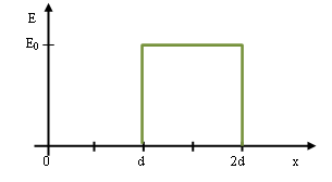
   The potentialdifference between the two points A and B is defined as

   V_B – V_A = –∫_A^B E•dl ,

   where dl is the parallel to the path of integration. The potential difference is independent of the path taken, so one may choose whichever path makes the integration easiest. If we take A as the point closer to the origin than B, then dl = i dx and then E•dl. = E dx. 

   V_B – V_A = –∫_A^B E dx

   Setting A at zero, and noting V(0) = 0, we have

   V_B =  –∫₀^B E dx .

   There are three distinct regions (see diagram above) where B could be. We need to do the above integral for each case. Note that the integrals may be piecewise.

   Region 1: 0 < B < d  

               We want the area under the graph from 0 to B where B is < d. Looking at the graph of E vs x, clearly this integral will be zero and thus V_B = 0.

   Region 2: d < B < 2d

   We want the area under the E vs x graph from 0 to B where B is less than 2d.

   

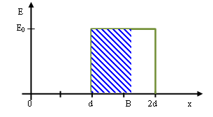
   We will need to break the integral into pieces

   V_B  =  –∫₀^B E dx = –∫₀^d E dx + –ò_d^B E dx = 0 – E₀(b – d) =  – E₀(B – d).

   Region 3: 2d < B

   We want the area under the E vs x graph from 0 to B where B is greater than 2D.

   

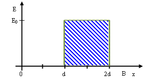
   We will need to break the integral into pieces

   V_B  =  –∫₀^B E dx = –∫₀^d E dx + –∫_d^2d E dx + –<∫_2d^B E dx = 0 – E₀(2d – d) – 0 =  – E₀d.

   Since point B can be any value of x, the potential looks like

   



---

8. Repeat the previous problem but take V = 0 at x = ∞.

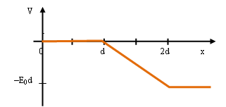
   Just like the previous question

   V_B – V_A = –∫_A^B E dx

   However, here we set B to infinity, and note V(∞) = 0, so that we get

   –V_A = –∫_A^∞ E dx .

   We will drop the minus signs from each side. There are three distinct regions (see diagram above) where A could be. We need to do the above integral for each case. Note that the integrals may be piecewise.

   Region 1: 0 < A < d

   We want the area under the graph from A to ∞ where A is < d. Looking at the graph of E vs x, clearly this integral include the entire area under the graph. The area is clearly E₀d but we will to break the integral into pieces.

   

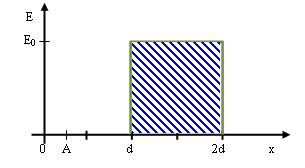
   V_A =  ∫_A^∞ E dx = ∫_A^d E dx +– ∫_d^2d E dx + ∫_2d^∞ E dx = 0 + E₀(2d – d) + 0 =  E₀d.

   Region 2: d < B < 2d

   We want the area under the E vs x graph from A to ∞ where A is less than 2d. We will need to break the integral into pieces.

   

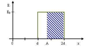
   V_A  =  ∫ _A^¥ E dx = ∫_A^2d E dx + ∫_2d^∞ E dx =  E₀(2d – A) + 0 = E₀(2d – A).

   Region 3: 2d < B

   Clearly in this region V_A = 0 since A is past 2d.

   Since point A can be any value of x, the potential looks like

   

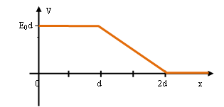
   The difference is that this graph is shifted upwards. Note that the difference in potential between any two points will be exactly the same as the previous question.



---



9. The electric field due to a uniformly charged long thick plate to be

   

   where d was the thickness of the plate, ρ₀ was the volume charge density, and x is the distance from the centre of the plate. Determine V(x) everywhere. Assume V(0) = 0. Plot V as a function of x.

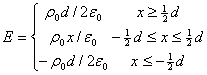
   The potential difference between the two points A and B is defined as

   V_B – V_A = – ∫_A^B E dx,

   where we have used E•dl = Edx. Setting A to be at zero and taking V_A = 0, we have

   V_B = –∫₀^BE dx .

   Since the electric field is symmetric, E(–x) = E(x), for this problem, then V(–x) = V(x).  Thus we only need to evaluate V(x) for two regions.

   (i)    For 0 ≤ B ≤ ½d

   VB	= –∫0B E dx
   	= –∫0B (ρ0/ε 0) x dx
   	= –(ρ0/ε0) ∫0B x dx
   	= –( ρ0 /ε 0) ½x2 |0B
   	= –( ρ0 B2 / 2 ε 0)

   (i)    For  B ≥ ½d

   VB	= – ∫0 B E(a)da
   	= –{ ∫0 ½d ( ρ0 /ε 0) x dx + ∫½d B ( ρ0 d/2ε 0) dx }
   	= –( ρ0 /ε 0) ∫0 ½d x dx – ( ρ0 d/2ε 0) ∫½d B dx
   	= –( ρ0 /ε 0) ½x2 |0½d – (ρ 0d/2 ε0 ) x |½dB
   	= –( ρ0 d2 / 8 ε 0) – ( ρ0 d/2ε 0)(B – ½d)
   	= –( ρ0 d/2ε 0)(B – ¼d)

   Since B can be any value of x, the potential looks like

   _A^B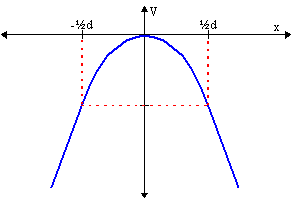

   Note that V(x) = 0 at x = 0, which is consistent with our assumption that V(0) = 0.



---

10. The electric field due to a long thin wire of uniform charge density λ to be E = (λ/2πε₀r)r where r is the radial distance from the wire and r is the unit radial vector. Determine V(r) relative to V(r=1) where r is the distance from the centre of the cylinder. Assume V(1) = 0. Plot V as a function of r.

    The potential difference between the two points B = r and A = 1 is defined as

    ΔV = V(r) − V(1) = −∫_A^B E · dl ,

    where dl is the parallel to the path of integration. The potential difference is independent of the path taken, so one may choose whichever path makes the integration easiest. We will integrate along the line joining the two points so that dl = rda, where r is the unit radial vector. Setting V(1) = 0, we have

    V(r) = −∫_A^B E · dl = −∫₁^r E r · r dr = −∫₁^r E dr .

    Evaluating V(r), we find

    V(r)	= −∫1r E dr
    	= −∫1r (λ/2ε0r) dr
    	= −(λ/2ε0) ∫1r dr/r
    	= −(λ/2ε0) ln(r) |1r
    	= −(λ/2ε0) ln(r)

    Note that V(r) is negative for r > 1 and positive for r < 1. The potential looks like

    

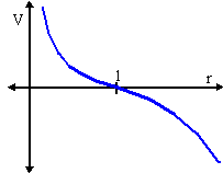
    Also note that V(r=1) = 0 consistent with our initial assumption.

    

    ---

11. The electric field due to a long thin cylindrical shell of radius R and negative surface charge density σ to be

    

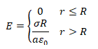
    where the field is radial (i.e. in the r direction). Determine V(r) relative to V(r = 0) where r is the distance from the centre of the cylinder. Assume V(0) = 0. Plot V as a function of r.

    The potential difference between the two points B = r and A = 0 is defined as

    ΔV = V(r) − V(0) = −∫_A^B E · dl ,

    where dl is the parallel to the path of integration. The potential difference is independent of the path taken, so one may choose whichever path makes the integration easiest. We will integrate along the line joining the two points so that dl = rda, where r is the unit radial vector. Setting V(0) = 0, we have

    V(r) = −∫_A^B E · dl = −∫₀^r E r · r dr = −∫₀^r E dr .

    Since E has two regions, we need to evaluate V(r) separately for each region.

    (i) For 0 ≤ r ≤ R

    V(r)	= −∫0r E dr
    	= −∫0r (0) dr
    	= 0

    (ii) For r ≥ R

    V(r)	= −∫0r E dr
    	= −∫0R E dr − ∫Rr E dr
    	= −∫0r (0) da − ∫Rr (σR/ε0) dr/r
    	= 0 − (σR/ε0) ln(r) |Rr
    	= − (σR/ε0) ln(r/R)

    The potential looks like

    

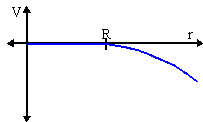
    Note that V(r=1) = 0 consistent with our initial assumption.

    

    ---

12. The electric field due to a solid sphere of radius R and total charge Q to be radial and have the form




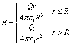
where the field is radial (i.e. in the r direction). Determine V(r) relative to V(∞) where r is the distance from the centre of the sphere. Assume V(r=∞) = 0. Plot V as a function of r.

The potential difference between the two points A = r and B = ∞ is defined as

ΔV = V(∞) − V(r) = −∫_A^B E · dl ,

where dl is the parallel to the path of integration. The potential difference is independent of the path taken, so one may choose whichever path makes the integration easiest. We will integrate along the line joining the two points so that dl = rd, where r is the unit radial vector. Setting V(∞) = 0, we have

−V(r) = −∫_A^B E · dl = −∫_r^∞ E r · r dr = −∫r^∞ E dr .

We can drop the minus sign from each side. Since E has two regions, we need to evaluate V(r) separately for each region.

(i) For 0 ≤ r ≤ R

V(r)	= ∫r∞ E dr
	= ∫rR E dr + ∫R∞ E dr
	=  ∫rR (Q/4πε0R3) rdr + ∫R∞ (Q/4πε0) dr/r2
	= (Q/4πε0R3) ½r2 |rR − (Q/4πε0) 1/r |R∞
	= (Q/8πε0R3)×(R2 − r2)  +  Q/4πε0R
	= 3Q/8πε0R − Qr2/8πε0R2

(ii) For r ≥ R

V(r)	= ∫r∞E dr
	= ∫r∞ (Q/4πε0) dr/r2
	= −(Q/4πε0) 1/r |r∞
	= Q/4πε0r

The potential looks like



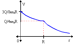
Note that V(r=∞) = 0, consistent with our initial assumption.



---

13. The electric field of a thick spherical shell of total charge Q and inner and outer radii of R and 2R to be



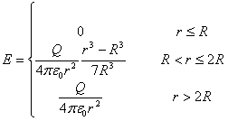
where the field is radial (i.e. in the r direction). Determine V(r) relative to V(∞)where r is the distance from the centre of the sphere. Assume V(∞) = 0. Plot V as a function of r.

The potential difference between the two points A = r and B = ∞ is defined as

ΔV = V(∞) − V(r) = −∫_A^B E · dl ,

where dl is the parallel to the path of integration. The potential difference is independent of the path taken, so one may choose whichever path makes the integration easiest. We will integrate along the line joining the two points so that dl = rdr, where r is the unit radial vector. Setting V(∞) = 0, we have

−V(r) = −∫_A^B E · dl = −∫_r^∞ E r · r dr = −∫_r^∞ E dr .

We drop the minus side from both sides. Since E has three regions, we need to evaluate V(r) separately for each region.

(i) For 0 ≤ r ≤ R

V(r)	= ∫r∞ E dr
	= ∫rR E dr  + ∫R2R E dr + ∫2R∞ E dr
	= ∫rR 0 dr + ∫R2R (Qr/28πε0R3−Q/28πε0r2) dr + ∫2R∞ (Q/4πε0) dr/r2
	= {(Q/28πε0R3) ½r2 + (Q/28πε0) 1/r }| R2R − (Q/4πε0) 1/r |2R∞
	= {(Q/560R3)(4R2 − R2) + (Q/28πε0)(1/2R − 1/R)} + Q/8πε0R
	= (9/14)( Q/4πε0R )

(ii) For R ≤ r ≤ 2R

V(r)	= ∫∞r E dr
	= ∫r2R E dr + ∫2R∞ E dr
	= ∫r2R (Qr/28πε0R3−Q/28πε0r2) dr + ∫2R∞ (Q/4πε0) dr/r2
	= {(Q/28πε0R3) ½r2 + (Q/28πε0) 1/r }| r2R − (Q/4πε0) 1/r |2R∞
	= {(Q/560R3)(4R2 − r2) + (Q/28πε0)(1/2R − 1/r)} + Q/8πε0R
	= (12/14)( Q/4πε0R) − (1/14)(Qr2/4πε0R3) − (2/14)(Q/4πε0r)

(iii) For r ≥ 2R

V(r)	=∫∞r E dr
	= ∫r∞ (Q/4πε0) dr/r2
	= −(Q/4πε0) 1/r |r∞
	= Q/4πε0r

The potential looks like



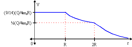
Note that V(r=∞) = 0, consistent with our initial assumption.



---

14. The electric field due to a thin spherical shell of radius R and surface charge −s to be



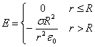
where the field is radial (i.e. in the r direction). Determine V(r) relative to V(r=∞) where r is the distance from the centre of the sphere. Assume V(r=∞) = 0. Plot V as a function of r.

The potential difference between the two points A = r and B = ∞ is defined as

ΔV = V(∞) − V(r) = −∫_A^B E · dl ,

where dl is the parallel to the path of integration. The potential difference is independent of the path taken, so one may choose whichever path makes the integration easiest. We will integrate along the line joining the two points so that dl = rdr, where r is the unit radial vector. Setting V(∞) = 0, we have

−V(r) = −∫_A^B E · dl = −∫_r^∞ E r · r dr = −∫_r^∞ E dr .

We will drop the minus sign from both sides. Since E has two regions, we need to evaluate V(r) separately for each region.

(i) For 0 ≤ r ≤ R

V(r)	= ∫r∞ E dr
	= ∫rR E dr + ∫R∞ E dr
	= ∫rR 0 dr + ∫R∞(σR2/ε0) dr/r2
	= −(σR2/ε0) 1/r |R∞
	= σR/ε0

(ii) For r ≥ R

V(r)	= ∫r∞ E dr
	= ∫r∞ (σR2/ε0) dr/r2
	= −(σR2/ε0) 1/r |r∞
	= σR2 / ε0r

The potential looks like



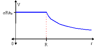
Note that V(r=∞) = 0, consistent with our initial assumption.



---

Potential of Point Charges

15. Two point charges of q₁ = 3.0 μC and q₂ = 4.0 μC are situated at the opposite corners of a rectangle as shown below. The short side has length L = 0.25 m. Find the total potential at points A and B. If a free particle of charge q_f = 1.0 μC and mass M = 15 g has speed v_A = 2.50 m/s at point A and it follows the indicated path, what will be its speed at point B?



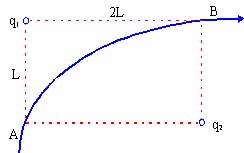
Points A and B are at different electrostatic potentials because of the arrangement of the charges. A positive charge will speed up if it moves from high potential to low or slow down if it moves from low potential to high. It does this because a high potential area has relatively more positive charge in the area than the low potential area and a positive charge is thus repelled.

So to find v_B, we find determine the potential at A and B. The potential at point A is given by the two fixed point charges and is equal to the sum of the potential of each charge

VA	= kq1/L + kq2/2L
	= (8.99 × 109 N−m2/C2)[(3 × 10−6C)/(0.25 m) + (3 × 10−6C)/(0.50 m)]
	= 1.798 × 105 Volts

Similarly the potential at point B is

VB	= kq1/2L + kq2/L
	= (8.99 × 109 N−m2/C2)[(3 × 10−6C)/(0.50 m) + (3 × 10−6C)/(0.25 m)]
	= 1.978 × 105 Volts

Using Conservation of Energy,

½m(v_B)² − ½m(v_A)² = q(V_A − V_B) .

Solving for v_B, we find

vB	= [(vA)2 + 2q(VA − VB)/m]½
	= [(2.50 m/s)2 + 2(1.00 × 10−6 C)(1.798105 − 1.978105 Volts)/(0.015 kg]½
	= 2.25 m/s



---

Electrostatic Energy of an Assemby of Point Charges


16. Five charges are arranged as shown below. What is the electrostatic potential energy of each configuration? The separation between charges is L.
 

The electrostatic potential of a charge configuration is given by the formula



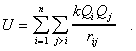
The charges in the diagrams below have been numbered and various value of r_ij have been shown.

(a)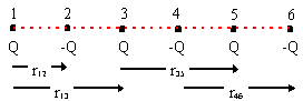 

U =	K(Q)(−Q)/L + K(Q)(Q)/2L + K(Q)(−Q)/3L + K(Q)(Q)/4L + K(Q)(−Q)/5L +  K(−Q)(Q)/L + K(−Q)(−Q)/2L + K(−Q)(Q)/3L + K(−Q)(−Q)/4L +  K(Q)(−Q)/L + K(Q)(Q)/2L + K(Q)(−Q)/3L +  K(−Q)(Q)/L + K(−Q)(−Q)/2L +  K(Q)(−Q)/L
=	−(35/12) KQ2/L

(b) 

U =	K(Q)(−Q)/L + K(Q)(Q)/2L + K(Q)(Q)/3L + K(Q)(Q)/4L + K(Q)(−Q)/5L +  K(−Q)(Q)/L + K(−Q)(Q)/2L + K(−Q)(Q)/3L + K(−Q)(−Q)/4L +  K(Q)(Q)/L + K(Q)(Q)/2L + K(Q)(−Q)/3L +  K(Q)(Q)/L + K(Q)(−Q)/2L +  K(Q)(−Q)/L
=	+(3/4) KQ2/L

In case (a) net energy was gained in assembling the charges while work had to be done to assemble the charges in (b). If left free to move, the charges in (a) would collapse in on themselves and would explode away from each other in (b).



---

Potential Due to a Distribution of Charge
17. (a) Find an integral expression for the electric potential at a point a distance a from one end of a long thin wire of length L and total charge Q. Examine the limit a >> L and show that your result is identical to that of a point charge.
    (b) If the charge distribution was λ(x) = 2Qx/L², where x = 0 is at the left side of the wire. Find an integral expression for the electric potential. Examine the limit a >> L and show that your result is identical to that of a point charge.
    

    (a) First we choose an origin. Part (b) mentions the left side of the wire, so we will use that. Second, we choose an abitrary infinitesmal piece of the wire dx having charge dq located arbitrary distance x from the origin. Third, we mark the vector that runs from dq to the point of interest. This is all shown in the next diagram.

    

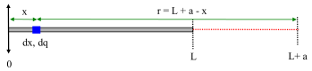
    The small piece of charge dq is related to the small wire of wire dx by the charge density λ = Q/L which gives dq = (Q/L)dx. The vector from the charge to the point of interest is r = i(L + a − x). We only need the magnitude r = L + a − x. Thus the integral for the potential is

    V = K ∫ dq/r = K ∫₀^L (Q/L)dx /(L + a − x).

    Note that the limits of integrations are the start and endpoints of the wire.

    Using a table of integrals, we can find

    V = −K (Q/L) ln(L + a − x) |₀^L = = −K (Q/L) ln[a/(L + a)] = K (Q/L) ln[(L + a)/a] = K (Q/L) ln[L/a + 1] .

    In the limit a >> L, ln[L/a + 1] ≈ L/a. Thus we get V = K (Q/L) × L/a = KQ/a which is the result for a point charge.

    (b) We are given a function for λ such that dq = 2(Q/L²)x dx. Thus the integral for the potential is

    V = K ∫ dq/r = 2K ∫₀^L (Q/L²)x dx /(L + a − x).

    Note that the limits of integrations are the start and endpoints of the wire.

    Using a table of integrals, we can find

    V = 2(KQ/L²) {(L + a)ln[(L + a)/a] − L}.

    In the limit a >> L, {(L + a)ln[(L + a)/a] − L} ≈ ½L/a. Thus we get V = 2(KQ/L) × ½L/a = KQ/a which is the result for a point charge.

    Note that we should make sure that Q was the charge on the wire in part (b). Q_Total = ∫₀^L dq = = ∫₀^L λ(x)dx = ∫₀^L 2(Q/L²) x dx = 2(Q/L²) × ½x² |₀^L = Q.

    

    ---

18. A total charge Q is distributed uniformly along a straight rod of length L. Find the potential at a point P at a distance h from the midpoint of the rod. (Hint: ∫[x²+k²]^−½dx = ln[x+[x²+k²]^½] + C). Use the gradient with respect to y to find the electric field at that point.



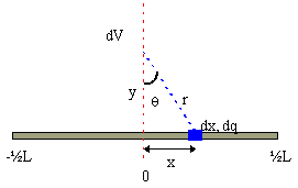
First, the wire has a uniform linear charge density = Q/L. Next, we consider a small portion of the wire, dx, located at a distance x from the left end of the wire having charge dq. These infinitesimals are related by

dq = dx = (Q/L)dx .

The electrostatic potential is a scalar given by

dV = kdq/r = k(Q/L)dx/r .

Before we can integrate, we need to find r in terms of x and y. Using trigonometry,

r = [y² + x²]^½ .

Hence

dV = (kQ/L)dx/[y² + x²]^½ .

Integrating over the entire length of the wire, we get the total potential to be

ΔV	= ∫−½L½L dV
	= (kQ/L) ∫−½L½L dx / [a2 + x2]½
	= (kQ/L) ln|x + [y2+x2]½| |−½L½L }
	= (kQ/L) ln|(½L + [y2+¼L2]½)/(−½L + [y2+¼L2]½)|

The electric field along the y−axis is given by

E_y = −j∂V /∂y = +j(KQ/y)[y²+¼L²]^−½ .

This is the same result as question 2 in the Gauss' Law handout.



---

19. Find an integral expression for the electric potential at a point midway between two long thin wires of length L and total charge Q and off to one side a distance h. The distance between the wires is a. The identity ∫[x²+k²]^-½dx = ln[x+[x²+k²]^½] + C may be of use. Use symmetry to simplify. Examine the limit h >> L.
    

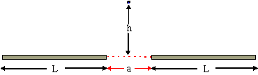
    Note that we have symmetry here. The contribution to potential from the lefthand wire is the same as that of the righthand wire. As a result, we find the potential just from the righthand side and double it.

    First we choose an origin; under the point of interest seems good. Second, we choose an abitrary infinitesmal piece of the wire dx having charge dq located arbitrary distance x from the origin. Third, we mark the vector that runs from dq to the point of interest. This is all shown in the next diagram.

    

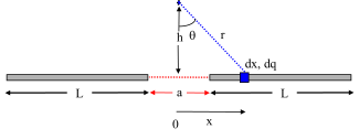
    The small piece of charge dq is related to the small wire of wire dx by the charge density λ = Q/L which gives dq = (Q/L)dx. The vector from the charge to the point of interest is r = −i(x − ½a) + jh. We only need the magnitude r = [(x − ½a)² + h²]^½. Thus the integral for the potential is

    V = 2 × K ∫ dq/r = 2K ∫_½a^L+½a (Q/L)dx /[(x − ½a)² + h²]^½.

    Note that the limits of integration are the start and endpoints of the wire.

    The integral becomes a little simpler if we do a change of variable z = x − ½a and then

    V = 2KQ/L ∫₀^L dz /[z² + h²]^½.

    Using a table of integrals, we can find

    V = 2KQ/L ln[z + [z² + h²]^½] |₀^L = 2KQ/L { ln[L + [L² + h²]^½] − ln(h) }

    In the limit h >> L, { ln[L + [L² + h²]^½] − ln(h) } ≈ L/h. Thus the potential reduces to V = 2KQ/h the result of being distance h from two point charges Q.



---

20. A wire of length 2L is bent in the centre to a right angle. It carries charge density λ. Find an integral expression for the electric potential at point P in the upper right corner of the diagram below. Use symmetry to simplify.
    

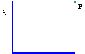
Note that we have symmetry here. The contribution to potential from the vertical wire is the same as that of the horizontaL wire. As a result, we find the potential just from the horizontal side and double it.

First we choose an origin; under the corner seems good. Second, we choose an abitrary infinitesmal piece of the wire dx having charge dq located arbitrary distance x from the origin. Third, we mark the vector that runs from dq to the point of interest. This is all shown in the next diagram.



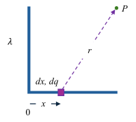
The small piece of charge dq is related to the small wire of wire dx by the charge density λ which gives dq = λdx. The vector from the charge to the point of interest is r = i(L − x) + jL. We only need the magnitude r = [(L − x)² + L²]^½. Thus the integral for the potential is

V = 2 × K ∫ dq/r = 2K ∫₀^L λdx /[(L − x)² + L²]^½.

Note that the limits of integration are the start and endpoints of the wire.

The integral becomes a little simpler if we do a change of variable z = x − L and dz =dx then

V = 2KQ/L ∫₀^L dz /[z² + h²]^½.

Using a table of integrals, we can find

V = 2KQ/L ln[z + [z² + L²]^½] |₀^L = 2KQ/L { ln[L + [L² + L²]^½] − ln(L) } = (2KQ/L) ln(1 + √2) .



---

21. Three thin rods of glass of length L carry charges uniformly distributed along their lengths. The charges on the three rods are +Q, +Q, and −Q, respectively. The rods are arranged along the sides of an equilateral triangle. What is the electrostatic potential at the midpoint of this triangle? (Hint: Use the result of the question 14.)



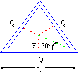
First we use trigonometry to find y in terms of L, y = L / 2tan(30°) = L / 2√3.

The potential of the triangle is the sum of the potentials due to its sides

V	= V1 + V2 + V3
	= (K/L)(Q + Q + −Q) ln|(½L + [y2+¼L2]½)/(−½L + [y2+¼L2]½)|
	= (KQ/L) ln|(L/2 + [L2/12+L2/4]½)/(−L/2 + [L2/12+L2+/4]½)|
	= (kQ/L) ln| (2 + √3) / (2 − √3)|

We could have arrived at this answer a little faster by noting that the −Q side would cancel with one of the +Q sides.



---

22. A rod is bent into a semi−circular arc of radius R. The rod has a uniform linear charge distribution λ. Find the potential at the centre of the arc, point P, by direct integration. The identity S= Rθ and dS = Rdθ may be of use.



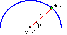
We consider a small portion of the wire, dS, with charge dq located at an angle θ, having charge dq. Note that angle θ must always be defined from the centre of curvature and measured counterclockwise from the positive x. The vector r is measured from dq to the centre of curvature. The magnitude is just R. These infinitesimals are related by

dq = λdS = Rdθ.

The electrostatic potential is a scalar given by

dV = kdq/R = kλdθ.

Integrating over the entire angular length of the wire, we get the total potential to be

ΔV	= ∫0πdV
	= (λk) ∫0πdθ
	= (πλk)

Note that the potential at the centre of the arc is independent of the radius of the arc. As well, since the potential of a point charge is set to be zero at r = ∞, and we built the arc out of point charge infinitesimals, this potential is also relative to infinity.



---

23. A thin semicircular wire of radius b has charge Q uniformly distributed along its length. Find an integral expression for the electric potential at a point P, a distance a horizontally from its centre. Use symmetry to simplify.
    

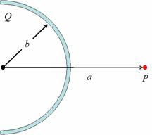
    We have some symmetry here. The upper half of the arc and the lower half of the arc make the same contribution to the potential. We will only find the contribution from the upper half and double it.

    We consider a small portion of the wire, dS, with charge dq located at an angle θ in the upper half having charge dq as shown in the diagram below. Note that angle θ must always be defined from the centre of curvature and measured counterclockwise from the positive x axis.

    

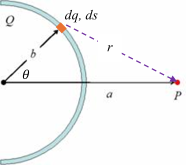
    The vector r is measured from dq to the point of interest P, r = i(a − bcosθ) − jbsinθ. The magnitude is just r = [(a − bcosθ)² + bsinθ²]^½. This can be simplified to r = [a² + b² − 2abcosθ]^½ which is the Cosine Law in trigonometry.

    These infinitesimals are related by

    dq = λdS = (Q/πb) bdθ = (Q/π) dθ.

    The integral we need to find is

    V = 2 × K ∫ dq/r = 2K ∫₀^π/2 (Q/π) dθ /[a² + b² − 2abcosθ]^½ = 2KQ/π ∫₀^π/2 dθ /[a² + b² − 2abcosθ]^½.

    The limits of integration correspond to the angular limits of the upper half of the wire.

    

    ---

24. A thin semicircular wire of radius b has charge density +λ on the upper half and opposite charge –λ on the lower half. Find the electric potential at the centre of curvature. Use symmetry to simplify.
    

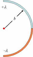
    For every infinitesmal small piece dq in the upper quarter circle, there is a symmetrical infinitesmal small piece −dq in the lower quarter circle which will cancel the contribution to the potential from the positive piece. The potential at the centre of curvature is zero.

    

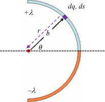
    Note that this would be true for any point along a horizontal axis passing through the centre of curvature. There would not be total cancellation for any other points.

    

    ---

E from V
 
25. The electric potential over a certain region is given by V = 3x²y−4xz−5y² volts. Determine the components of the electric field and evaluate at the point (+1,0,+2).
 

The electric field is given by the negative gradient of the electrostatic potential

E	= −∇V
	= −i∂V /∂x + −j∂V/∂y + −k∂V/∂z
	= −i(6xy − 4z) + −j(3x2 − 10y) + −k(−4x)

At (1,0,2) the electric field is

E = 8i − 3 j + 4k.



---

26. Over a certain region of space, the electric potential is V = 5x−3x²y+2yz². Determine the components of the electric field and evaluate electric field at the point (1,0,−2).



The electric field is given by the negative gradient of the electrostatic potential

E	= −∇V
	= −i∂V/∂x + −j∂V/∂y + −k∂V/∂z
	= −i(5 − 6xy) + − j(−3x2 + 2z2) + −k(4yz)

At (1,0,−2) the electric field is

E = −5i − 5j .

Questions? mike.coombes@kpu.ca