Questions: 1 2 3 4 5 6 7 8 9 10 11

Induction - Faraday's Law and Lenz' Law Solutions

1. The diagram below shows a uniform magnetic field confined to a cylindrical region of space (seen end on). The magnitude of the field is B = 1.72 T. The circular cross-section of the region has a radius of 0.10 m. The magnetic field is also shown with three different square regions. The sides of the square regions are L₁ = L₂ = 0.30 m and L₃ = 0.10 m.
   (a) Find the flux in each square region.
   (b) If the flux is increasing 0.025 T/s, what is the induced emf around the perimeter of each square region–

   

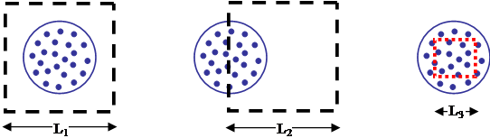
   (a) Magnetic flux is defined by Φ_m = BAcos(θ), where the angle θ is between the direction of the magnetic field B and a unit vector perpendicular to the area of interest. In this problem B is out of the page and so is the vector normal to the squares. Thus θ = 0 and cos(0) = 1.

   We need to be careful about area A. It is the area that contains magnetic field. For the first square, side L₁, only the circle actually carries flux. So

   Φ₁ = Bπr² = (1.72 T)π(0.10 m)² = 0.05404 T-m² .

   For the second square only half the circle is enclosed, so

   Φ₂ = ½Bπr² = ½(0.0504 T-m²) = 0.02702 T-m² .

   For the third small square, we need to ignore the field outside of the square. Hence here A is the size of the small square

   Φ₃ = BL₃²  = (1.72 T)(0.10 m)² = 0.0172 T-m² .

   (b) Since only the magnetic field is changing, the emfs are

   ε₁ =  –(dB/dt)πr² = –(0.025 T/s)π(0.10 m)² = –7.854 × 10^-4 T-m²/s ,

   ε₂ =  –(dB/dt)½πr² = –(0.025 T/s)½π(0.10 m)² = –3.9270 × 10^-4 T-m²/s , and

   ε₁ =  –(dB/dt) L₃² = –(0.025 T/s) (0.10 m)² = –2.50 × 10^-4 T-m²/s .



---

2. In the diagram below, a circular loop is in a uniform magnetic field B = 0.045 T. The field is oriented at an angle of θ = 25° to normal to the loop. The radius of the loop is 10 cm.
   (a) Find the magnetic flux through the loop.
   (b) If the magnetic field decreases at a rate of 0.050 T/s, find the induced emf in the loop.
   (c) If, instead, the radius of the loop increases at 0.10 m/s, find the induced emf in the loop.
   (d) If direction of the magnetic field increases at the rate of 2.5 rad/s find the induced emf in the loop.
   (e) If all the above changes occur at the same time, find the induced emf in the loop.
   (f) Which way would a current flow in each case.
   

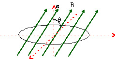
   (a) Magnetic flux is defined by,
   

   Φm = BAcos(θ) .

   (1)

   Evaluating the flux for the given data,
   

   Φm	= BAcos(θ)
   	= (0.45 T)π(0.1 m)2cos(25°)
   	= 1.28 × 10-3 Tm2

   From Faraday's Law, the induced emf is
   

   ε = -dΦm/dt .

   (2)

   Applying (2) to (1) yields
   

   ε = -(dB/dt)Acos(θ) - B(dA/dt)cos(θ) + BAsin(θ)(dθ/dt) .

   (3)

   Now the area of a circular loop is A = πr², so equation (3) becomes
   

   ε = -(dB/dt)Acos(θ) - 2rB(dr/dt)cos(θ) + BAsin(θ)(dθ/dt).

   (4)

   (b) If only B is changing, dB/dt = -0.05 T/s and dr/dt = dθ/dt = 0. We get

   ε	= -(dB/dt)Acos(θ)
   	= -(-0.050 T/s)π(0.1 m)2cos(25°)
   	= +1.42 × 10-3 Volts

   (c) If only r is changing, dr/dt = +0.10 m/s and dB/dt = dθ/dt = 0. We get

   ε	= -2rB(dr/dt)cos(θ)
   	= -2(0.1 m)(0.045 T)(0.010 m/s)cos(25°)
   	= -2.56 × 10-3 Volts

   (d) If only is changing, dθ/dt = +2.5 rad/s and dB/dt = dr/dt = 0. We get

   ε	= +BAsin(θ)(dθ/dt)
   	= +(0.045 T)π(0.1 m)2sin(25°)(2.5 rad/s)
   	= +1.49 × 10-3 Volts

   (e) If all variables are changing at once, the result is the sum of the answers from (b) to (d).

   ε	= -(dB/dt)Acos(θ) - 2rB(dr/dt)cos(θ) + BAsin(θ)(dθ/dt)
   	= +1.42 × 10-3 Volts - 2.56 × 10-3 Volts + 1.49 × 10-3 Volts
   	= +3.5 × 10-4 Volts

   (f) We need to establish a coordinate system. In the diagram below, we show the coil as if we were looking down at it. The magnetic field is initially out of the page.

   

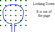
   Lenz's Law state the current will be such to oppose the change. If B out through the loop is increasing, the current will be such to create flux into the page. This requires a clockwise current. If B out through the loop is decreasing, the counterclockwise current will be such to create flux out of the page.
   

   In (b) B out of the page is decreasing, so the current is CCW. In (c), the area is increasing so the amount of flux though the loop is increasing. Hence the current is CW. In (d) the flux decreases as θ goes to 90°. Thus the current is CCW. In (e), the sign of is the same as in (b) and (d) so the current is in the same direction, CCW.

   

   ---

3. A single circular hoop moves with constant velocity through regions where uniform magnetic fields of the same magnitude are directed either into or out of the plane of the page as indicated below. Determined the direction of the induced current, if any, at each of the seven marked positions. HINT: sketch the flux as a function of position.

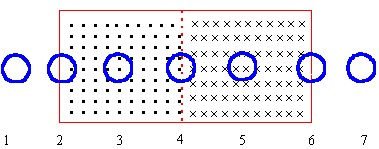
   At points (1), (3), (5), and (7) the flux is constant (zero) and no emf or current is produced.
   

   At (2) the flux out of the page through the loop is increasing. The emf and current are such to counter the growth by generating flux into the page. The current will be CW by the right hand rule.
   

   At (4) the flux out of the page through the loop is decreasing. The emf and current are such to counter the decrease by generating flux out of the page. The current will be CCW by the right hand rule.
   

   At (6) the flux into the page through the loop is decreasing. The emf and current are such to counter the decrease by generating flux into the page. The current will be CW by the right hand rule.
   



---

4. A square 0.1 m × 0.1 m metal coil is travelling at v = 1 m/s toward a region of space with two magnetic fields side by side. The regions are each 0.4 m wide. In the first region, the magnetic field is a constant 0.9 T directed out while the field is a constant 0.9 T inward in the second region.
   (a) Plot Φ vs t where t = 0 is when the square first reaches the magnetic field region. Label the axes!
   (b) Plot ε vs t where t = 0 is when the square first reaches the magnetic field region. Label the axes!
   (c) How would your answers change if the coil is travelling at v = 2 m/s?
   

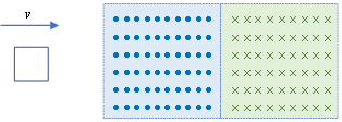
   (a) The first step in plotting Φ vs t is to determine when the square coil is at a boundary as shown in the diagram below.

   

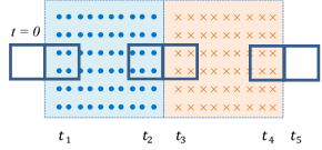
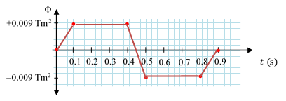
   Since the square coil is travelling at a constant speed, at time t₁ it has travelled d = 0.1 m. So t₁ = d/v = (0.1 m)/(1 m/s) = 0.10 s. Similarly, t₂ = (0.4 m)/(1 m/s) = 0.40 s, t₃ = (0.5 m)/(1 m/s) = 0.50 s, t₄ = (0.8 m)/(1 m/s) = 0.80 s, and t₅ = (0.9 m)/(1 m/s) = 0.90 s. At t₁ and t₂, the flux is Φ = BA = (0.9 T)(0.1 m×0.1 m) = +0.009 Tm² where the + indicates that the flux is out of the page. Similarly at t₃ and t₄, the flux is Φ = −0.009 Tm² where the − indicates that the flux is into the page . There is no flux through the coil at t₅ or t = 0.

   We next plot the values of Φ at the appropriate times and join the points by straight lines since the velocity is constant. This is shown in the next diagram.

   

   (c) The induced emf is given by ε = -dΦ/dt. In terms of the above graph, it is the negative of the slopes of the line segments. The slope of the first and last line segment is (0.009)/(0.10), so the emf is ε = −0.090 V. The slope of the middle segment is (−0.018)/(0.10), so the emf is ε = 0.180 V. The flat segments have zero slope and no emf is induced. A plot of these results is given in the diagram below.

   

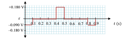
   Note that the direction of emf can be determined from Lenz’ Law. As the square coil moves into the magnetic field, the flux out through the coil is increasing. The coil responds with and emf into the page or CW. As the coil moves from the B_out to the B_in region, the flux out is decreasing, so the induced emf is out of the page or CCW.

   (c) Doubling the speed decreases the time spent in each region by half. As a result, the slopes all double as does the induced emf.

   

   ---

5. A square 0.1 m × 0.1 m metal coil is travelling at v = 1 m/s toward a region of space with two magnetic fields side by side. The regions are each 0.4 m wide. In the first region, the magnetic field is a constant 0.9 T directed out while the field is a constant 0.9 T inward in the second region. The second region is 0.05 m high and is centered on the oncoming coil.
   (a) Plot Φ vs t where t = 0 is when the square first reaches the magnetic field region. Label the axes!
   (b) Plot ε vs t where t = 0 is when the square first reaches the magnetic field region. Label the axes!
   

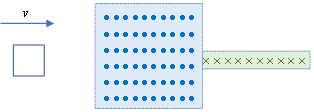
   (a) The first step in plotting Φ vs t is to determine when the square coil is at a boundary as shown in the diagram below.

   

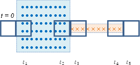
   Since the square coil is travelling at a constant speed, at time t₁ it has travelled d = 0.1 m. So t₁ = d/v = (0.1 m)/(1 m/s) = 0.10 s. Similarly, t₂ = (0.4 m)/(1 m/s) = 0.40 s, t₃ = (0.5 m)/(1 m/s) = 0.50 s, t₄ = (0.8 m)/(1 m/s) = 0.80 s, and t₅ = (0.9 m)/(1 m/s) = 0.90 s. At t₁ and t₂, the flux is Φ = BA = (0.9 T)(0.1 m×0.1 m) = +0.009 Tm² where the + indicates that the flux is out of the page. Similarly at t₃ and t₄, the flux is Φ = −0.009 Tm² where the − indicates that the flux is into the page . There is no flux through the coil at t₅ or t = 0.

   We next plot the values of Φ at the appropriate times and join the points by straight lines since the velocity is constant. This is shown in the next diagram.

   

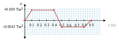
   (b) The induced emf is given by ε = -dΦ/dt. In terms of the above graph, it is the negative of the slopes of the line segments. The slope of the first line segment is (0.009)/(0.10), so the emf is ε = −0.090 V. The slope of the middle segment is (−0.0135)/(0.10), so the emf is ε = +0.135 V. The slope of the first last line segment is (0.0045)/(0.10), so the emf is ε = −0.045 V. The flats segments have zero slope and no emf is induced. A plot of these results is given in the diagram below.

   

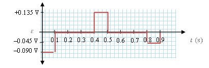
   Note that the direction of emf can be determined from Lenz’ Law. As the square coil moves into the magnetic field, the flux out through the coil is increasing. The coil responds with an emf into the page or CW. As the coil moves from the B_out to the B_in region, the flux out is decreasing, so the induced emf is out of the page or CCW.

   

   ---

6. An L-shaped metal coil is travelling at v = 2 m/s toward a region of space with a magnetic field. The region is 0.4 m wide. The magnetic field is a constant 0.8 T directed outward. The L-shape is 0.10 m on the long sides and 0.05 m on the short sides.
   (a) Plot Φ vs t where t = 0 is when the square first reaches the magnetic field region. Label the axes!
   (b) Plot ε vs t where t = 0 is when the square first reaches the magnetic field region. Label the axes!
   

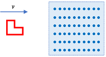
   (a) The first step in plotting Φ vs t is to determine when the L-shaped coil is at a boundary, or when the smaller square of the shape is at a boundary, as shown in the diagram below. The shapes are shifted vertically so that they can all be seen easily

   

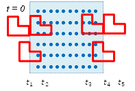
   Since the square coil is travelling at a constant speed, at time t₁ it has travelled d = 0.050 m. So t₁ = d/v = (0.050 m)/(2 m/s) = 0.025 s. Similarly, t₂ = (0.1 m)/(2 m/s) = 0.050 s, t₃ = (0.4 m)/(2 m/s) = 0.200 s, t₄ = (0.45 m)/(2 m/s) = 0.225 s, and t₅ = (0.5 m)/(2 m/s) = 0.250 s. At t₁ the flux is Φ = BA = (0.8 T)(¼)(0.1 m × 0.1 m) = +0.002 Tm² where the + indicates that the flux is out of the page. At t₂ and t₃, the flux is Φ = BA = (0.8 T)(¾)(0.1 m × 0.1 m) = +0.006 Tm². At t₄ the flux is Φ = BA = (0.8 T)(½)(0.1 m × 0.1 m) = +0.002 Tm². There is no flux through the coil at t₅ or t = 0.

   We next plot the values of Φ at the appropriate times and join the points by straight lines since the velocity is constant. This is shown in the next diagram.

   

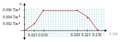
   (b) The induced emf is given by ε = -dΦ/dt. In terms of the above graph, it is the negative of the slopes of the line segments. The slope of the first line segment is (0.002)/(0.025), so the emf is ε = −0.080 V. The slope of the second line segment is (0.004)/(0.025), so the emf is ε = −0.160 V. The slope of the third segment is zero as is the induced emf. The slope of the fourth segment is (−0.002)/(0.025), so the emf is ε = +0.080 V. The slope of the last line segment is (−0.004)/(0.025), so the emf is ε = +0.160 V. A plot of these results is given in the diagram below.

   

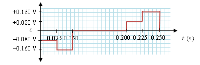
   Note that the direction of emf can be determined from Lenz’ Law. As the L-shaped coil moves into the magnetic field, the flux out through the coil is increasing. The coil responds with an emf into the page or CW. As the coil moves out of the field , the flux out is decreasing, so the induced emf is out of the page or CCW.

   

   ---

7. A square 0.1 m × 0.1 m metal coil is at rest just at the edge a region of space with a magnetic field of 0.8 T out. The region is 0.4 m wide. At t = 0 s, the coil accelerates forward with a = 2 m/s².
   (a) Determine Φ as a function of time.
   (b) Determine ε as a function of time.
   

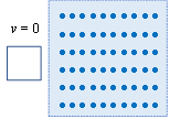
   (a) The first step in plotting Φ vs t is to determine when the square coil is at a boundary as shown in the diagram below.

   

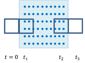
   Since the square coil is accelerating from rest, we find the travel time from the kinematics formula d = ½at² or t = √(2d/a). Since it has travelled d = 0.1 m at t₁, t₁ = √(0.1) = 0.316 s. Similarly, it has travelled d = 0.4 m at t₂, t₂ = √(0.4) = 0.632 s. Finally, it has travelled d = 0.5 m at t₃, t₃ = √0.5=0.707 s. At t₁ and t₂, the flux is Φ = BA = (0.8 T)(0.1 m×0.1 m) = +0.008 Tm² where the + indicates that the flux is out of the page. There is no flux through the coil at t₃ or t = 0.

   We next plot the values of Φ at the appropriate times. The flux is constant between t₁ and t₂ and we may join the data points by straight line. However, since the velocity is not constant, the data points at t = 0 and t₁ and the datapoints at t₂ and t₃ must be joined by curves. This is shown in the next diagram.

   

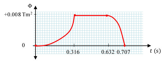
   (b) The induced emf is given by ε = −dΦ/dt. In terms of the above graph, it is the negative of the slopes of the tangents to the curves. This is hard to do and we must instead find an expression for the flux as a function of time so that we may differentiate. However, the flat segment has zero slope and no emf is induced.

   To determine an expression for the flux, it is helpful to have a picture of the coil crossing a boundary as shown in the diagram below.

   

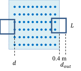
   For the entry, Φ = BA = BLd where d = ½at². So Φ = ½BLat². For the exit, Φ = BA = BL(L − (d_out − 0.4)) = BL(L + 0.4 − ½at²). Now that we have equations for the flux, we find ε_entry = −dΦ/dt = −BLat = −(0.8)(0.1)(2)t = −0.16t. This is linear with a value of ε = 0 at t = 0 and ε = −0.0506 V at t₁ = 0.316 s. For the exit, we have ε_exit = −dΦ/dt = +BLat. At t₂ = 0.632 s, this is ε_exit = (0.8)(0.1)(2)t = 0.1012 V. At t₃ = 0.707 s, this is ε_exit = 0.1131 V. A plot of these results is given in the diagram below.

   

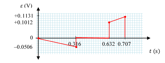
   Note that the direction of emf can be determined from Lenz’ Law. As the square coil moves into the magnetic field, the flux out through the coil is increasing. The coil responds with and emf into the page or CW. As coil exits the field, the flux out is decreasing, so the induced emf is out of the page or CCW.

   

   ---

8. In diagram (a) below, an equilateral triangle is just entering, at time t =0, a region of constant magnetic field B = 0.335 T into the page. In diagram (b) at some later time t > 0, the triangle has moved a distance x into the magnetic field. The triangle has sides of length L = 1.20 m long and is moving to the right at constant speed v = dx/dt = 2.50 m/s.
   (a) Derive an expression for the magnetic flux Φ_m as a function of x. Hints: The area of a triangle is one-half the base times the height. Consider similar triangles.
   (b) What is the magnitude of the induced emf at t = 0.30 s?
   (c) What is the direction of the induced emf at t = 0.30 s– Fully explain your reasoning.
   (d) If the resistance of the wire is 0.50 Ω, what is the current in the wire?
   

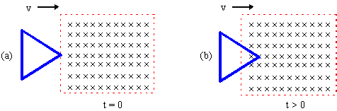
   (a)Magnetic flux is defined by,
   

   Φm = BAcos(θ) .

   (1)

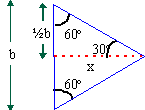
   Here A is the area of the triangle that is in the magnetic field B. The triangle is perpendicular to the field so θ = 0 and cos(0) = 1. We will use a little geometry to find that area. Examining the diagram below, we see that A = ½bx. However we need to express b in terms of x. We have a right triangle so tan(30°) = b/2x and hence b = 2xtan(30°) = 2x/√3. Thus A = x²/√3.
   

   

   Therefore
   

   Φm = Bx2/√3 .

   (3)

   (b) The emf produced is given by Faraday's Law
   

   ε = -dΦm/dt .

   (3)

   Differentiating (2) yields

   ε = -(2/√3)Bx dx/dt .

   (4)

   Now v = dx/dt and x = vt for constant speed, so (4) becomes
   

   ε = -(2/√3)Bv2t .

   (5)

   Evaluating for the given data yields
   

   ε = -(2/√3)(0.355 T)(2.50 m/s)²(0.30 s) = -0.77 Volts .

   (b) The flux down through the loop is increasing. Lenz's Law says that the emf and current produced will counteract this by generating flux up through the loop. By the right hand rule, the emf and current are CCW.
   

   (c) Using Ohm's Law, the current in the loop is

   I = ε/R = 0.77 V / 0.50 = 1.54 Amps .

   

---

9. The DC-10 jet aircraft has a wingspan of 47 m. If such an aircraft is flying horizontally at 960 km/h at a place where the vertical component of the earth's magnetic field is 60 μT, what is the induced emf between its wingtips?
   

   We know that the emf produced in a conductor moving through a magnetic field at right angles is

   ε	= ℓ v B⊥
   	= (47 m)(960 km/h × 1000 m/km × 1 h /3600 s) (60 × 10-6 T)
   	= 0.75 Volts

   

---

10. The diagram below shows three 1.0 m long, thin rods moving at v = 100 m/s through a magnetic field of strength B = 0.75 T out of the page. Find the motional emf in each case.
    

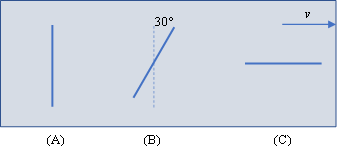
    (A) Each of ℓ, v, and B are perpendicular to one another, so ε = ℓ v B = (1.0 m) (100 m/s) (0.75 T) = 75.0 V.

    (B) The rod is travelling at an angle to the magnetic field v. Only the portion of the rod perpendicular to v contributes, ε = ℓ cos(30°) v B = (1.0 m)(cos(30°)) (100 m/s) (0.75 T) = 65.0 V.

    (C) The rod is parallel to v, there will be no motional emf, ε = 0.

    

---

11. Two parallel conducting rails are inclined at 30 degrees to the horizontal, and are joined at the top by a length of copper wire; the rails and wire have negligible resistance. A 0.40 m long conducting rod of resistance 2.00 Ω slides without friction down the rails. Sliding through the magnetic field induces a current in the rod. The current-carrying rod then experiences a force from the external magnetic field. Assuming that the component of the magnetic field perpendicular to the incline, B_⊥, points up, what magnitude must it have to ensure that the rod slides with a constant velocity of 5.00 m/s. The mass of the rod is 50.0 g. If the perpendicular component of the magnetic field pointed down what effect would this have? Why can we neglect the parallel component of the magnetic field, B_||?

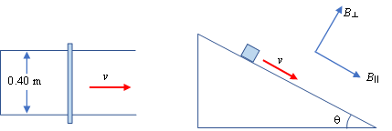
    Only B_⊥ has an effect because B_|| is in the same direction as the motion. Faraday's Law states that an emf is produced only when field lines are crossed.
    

    The magnitude of the produced emf is ε = vLB_⊥, for a rod moving through a magnetic field. If we examine the diagram above, the area swept out by the rod is increasing. Therefore the flux through this area is also increasing out of the page. According to Lenz's Law, the emf produced must be CW to create a flux into the page. Since there is a conducting path there will be a CW current as well. Using Ohm's Law, the current will have a magnitude I = ε/R = vLB_⊥/R .
    

    We also know that a current carrying wire moving through a magnetic field will experience a magnetic force F_m = ILB_⊥ = v(LB_⊥)²/R. Using the right hand rule, the force is directed up the incline.
    

    We are told that the velocity of the rod is constant so a = 0. Let's draw the free body diagram and apply Newton's Second Law.
    

    

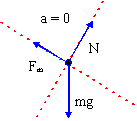
    We get

    ΣFx	= max		ΣFy	= may
    -Fm + mgcos(θ)	= 0		N - mgsin(θ)	= 0

    So we get
    

    v(LB_⊥)²/R = mgcos(θ) .

    Solving for B_⊥, we find
    

    B⊥	= [Rmgsin(θ) / vL2]½
    	= [(2 Ω)(0.050 kg)(9.81 m/s2)sin(30°) / (5 m/s)(0.40 m)2]½
    	= 0.78 T

    If the B were down instead of up, the current would circulate CCW. The magnetic force would still be up the incline, so the magnitude of B would remain the same.
    

    

Questions– mike.coombes@kpu.ca