![[Return to Physics Homepage]](../../physics.gif)
![[Return to Mike Coombes' Homepage]](../../coombes.gif)
![[Return to List of Handouts]](../../handouts.gif)
![[Return to List of Notes and Examples]](../../notes.gif)
Uncertainty is intrinsic to measurement. Doing a calculation with measured quantities requires an understanding of how the uncertainties effect or propagate through the calculation.
Uncertainties may be written in absolute or relative terms
a ± δa or a ± &alpha% ,
where α = (δa/a) × 100.
The uncertainty δa/a or α should be given to one significant digit. There is no difference between the two forms. However, you may be required to present your results in one form rather than the other.
We distinguish between uncertain quantities and exact quantities such a π or 2.2 that have no uncertainty. Exact quantities may be represented as a point on a number line whereas uncertain quantities are represented by a line segment. Figure 1 below shows the exact quantity 1.3 and the uncertain quantity 1.3 <± 0.4 .

The key to error propagation is understanding that we are dealing with a range of numbers, and that any calculation will produce a range of values as an answer, from the smallest that the answer could be to the largest. As a simple example consider the difference between adding two exact quantities, for example adding 4.5 to 3.8, compared to adding 4.5 <± 0.2 to 3.8 <± 0.4. The exact result is 4.5 + 3.8 = 8.3 . The smallest answer we can get for the uncertain quantities is (4.5-0.2) + (3.8-0.4) = 7.7 . The largest answer we can get is (4.5+0.2) + (3.8+0.4) = 8.9 . We would state the answer for the range as 8.3 <± 0.6 .
Simple addition with uncertain quantities is easy to do, but throw in other operations like multiplication and functions like cosine, and things get complicated fast. Luckily there are a few rules that we can use to make these calculations simpler. The rules are usually approximations and are based on the assumption that the relative uncertainty in any one number is small, say under 10%, so the precision of all your measurements must be that high.
When we do mathematical operations such as addition or multiplication with measured quantities, we are looking for both the principle value of the result as well as the maximum uncertainty. For example, consider
A + B = P(A + B) ± δ(A + B)
P(A+B) is the principle value of the sum A + B, the value found when the uncertainty in neglected. Here P(A+B) is 4.5 + 3.8 = 8.3. δ(A + B) is the maximum uncertainty in the sum A + B, which we already found to be 0.2 + 0.4 = 0.6.
Warning! This notation is not standard. As an example, considered the product A × B.
A × B = P(AB) ± δ(AB)
As we will see later, this is
A × B = P(AB) <± P(AB)[δ(A)/P(A) + δ(B)/P(B)]
It is common, if sometimes misleading, to see the above written as
A × B = AB <± (AB)(δA/A + δB/B)
In the above A refers to both the measured value and its principle value and δA refers to the uncertainty in A. Unfortunately, this "sloppy" notation is close to being the standard.

Derivation of Rule for Addition
This result can be derived quite simply. First, consider the addition of two measurements
A + B = [P(A) ± δ(A)] + [P(B) ± δ(B)]
- Finding the maximum possible value when adding
The biggest this sum can be is
[P(A) + δ(A)] + [P(B) + δ(B)] = P(A + B) + [δ(A) + δ(B)]
- Finding the minimum possible value when adding
The smallest this sum can be is
[P(A) - δ(A)] + [P(B) - δ(B)] = P(A + B) - [δ(A) + δ(B)]
- Result for addition
Combining the result for the maximum and minimum values, the range of values for addition is
[P(A) ± δ(A)] + [P(B) ± δ(B)] = P(A + B) <± [δ(A) + δ(B)]
It should be clear that no matter how many numbers we add together, we should get the general result
[P(A1) ± δ(A1)] + [P(A2) ± δ(A2)] + ... + [P(An) ± δ(An)] = P(A1 + A2 + ... + An) <± [δ(A1) + δ(A2) + ... + δ(An)]
So the maximum uncertainty in the sum A1 + A2 + ... + An is
δ(A1 + A2 + ... + An) = [δ(A1) + δ(A2) + ... + δ(An)] = δa1 + δa2 + ... + δan
In "sloppy" notation, this is
δ(A1 + A2 + ... + An) = δA1 + δA2 + ... + δAn
Derivation of Rule for Subtraction
Next, consider the subtraction of two measurements
A - B = [P(A) ± δ(A)] - [P(B) ± δ(B)]
- Finding the maximum possible value when subtracting
The biggest this difference can be is
[P(A) + δ(A)] - [P(B) - δ(B)] = P(A - B) + [δ(A) + δ(B)]
- Finding the minimum possible value when subtracting
The smallest this difference can be is
[P(A) - δ(A)] - [P(B) + δ(B)] = P(A - B) - [δ(A) + δ(B)]
- Result for subtraction
Combining the result for the maximum and minimum values, the range of values for subtraction is
[P(A) ± δ(A)] - [P(B) ± δ(B)] = P(A - B) <± [δ(A) + δ(B)]
It should be clear that no matter how many numbers we subtract, we should get the general result
[P(B1) ± δ(B1)] - [P(B2) ± δ(B2)] - ... - [P(Bn) ± δ(Bn)] = P(B1 - B2 - ... - Bn) <± [δ(B1) + δ(B2) + ... + δ(Bn)]
So the maximum uncertainty in the difference B1 - B2 - ... - Bn is
δ(B1 - B2 - ... - Bn) = [δ(B1) + δ(B2) + ... + δ(Bn)] = δb1 + δb2 + ... + δbn
In "sloppy" notation, this is
δ(B1 - B2 - ... - Bn) = δB1 + δB2 + ... + δBn
Note that whether we are adding or subtracting, we add absolute uncertainties.
Example
Let A = 5.23 <± 0.07, B = 4.67 <± 0.04, and C = 7.11 <± 0.09. Find F = A + B - C.
First
P(F) = P(A + B - C) = 5.23 + 4.67 - 7.11 = 2.79
Next, using our rule
| δ(F) | = δ(A + B - C) |
| = δ(A) + δ(B) + δ(C) | |
| = 0.07 + 0.04 + 0.09 | |
| = 0.20 |
Thus the answer is
F = 2.79 <± 0.20
We can only keep one figure in the uncertainty, thus
F = 2.8 <± 0.2

Derivation of Rule for Multiplication
This result can be derived as follows. First, consider the multiplication of two measurements
A × B = [P(A) ± δ(A)] × [P(B) ± δ(B)]
- Finding the maximum possible value when multiplying
The biggest the product AB can be is
[P(A) + δ(A)] × [P(B) + δ(B)] = P(AB) + [P(B)δ(A) + P(A)δ(B) + δ(A)δ(B)]
Now δ(A) and δ(B) are supposed to be small compared to P(A) and P(B). As well we keep the uncertainty only to one figure. Hence δ(A)δ(B) is negligible and can be dropped. Thus we have
[P(A) + δ(A)] × [P(B) + δ(B)] = P(AB) + [P(B)δ(A) + P(A)δ(B)]
We usually rewrite the above expression as
[P(A) + δ(A)] × [P(B) + δ(B)] = P(AB) + P(AB)[δ(A)/P(A) + δ(B)/P(B)]
- Finding the minimum possible value when multiplying
The smallest the product AB can be is
[P(A) - δ(A)] × [P(B) - δ(B)] = P(AB) - [P(B)δ(A) + P(A)δ(B) + δ(A)δ(B)]
Now δ(A) and δ(B) are supposed to be small compared to P(A) and P(B). As well we keep the uncertainty only to one figure. Hence δ(A)δ(B) is negligible and can be dropped. Thus we have
[P(A) - δ(A)] × [P(B) - δ(B)] = P(AB) - [P(B)δ(A) + P(A)δ(B)]
We usually rewrite the above expression as
[P(A) - δ(A)] × [P(B) - δ(B)] = P(AB) - P(AB)[δ(A)/P(A) + δ(B)/P(B)]
- Result for multiplication
Combining the result for the maximum and minimum values, the range of values for multiplication is
A × B = [P(A) ± δ(A)] × [P(B) ± δ(B)] = P(AB) <± P(AB)[δ(A)/P(A) + δ(B)/P(B)]
Remember that this result is an approximation, good only when the relative uncertainties are small.
When we multiply many numbers, the pattern is the same
| A1 × A2 × ... × An = | [P(A1) ± δ(A1)] × [P(A2) ± δ(A2)] × ... × [P(An) ± δ(An)] |
| = | P(A1A2 ... An) <± P(A1A2 ... An)[δ(A1)/P(A1) + δ(A2)/P(A2) + ... + δ(An)/P(An)] |
So the maximum uncertainty in the product A1 × A2 × ... × An is
δ(A1 × A2 × ... × An) = (a1a2 ... an) [δa1/a1 + δa2/a2 + ... + δan/an]
In "sloppy" notation, this is
δ(A1 × A2 × ... × An) = (A1A2 ... An) [δA1/A1 + δA2/A2 + ... + δAn/An]
Derivation of Rule for Division
Next consider the division of two measured quantities
A/B = [P(A) ± δ(A)] / [P(B) ± δ(B)]
First we rewrite this in relative form as
[P(A)(1 ± δ(A)/P(A))] / [P(B)(1 ± δ(B)/P(B))] = P(A/B) × [1 ± δ(A)/P(A)]/[1 ± δ(B)/P(B)]
- Finding the maximum possible value for division
The biggest A/B can be is
P(A/B) × [1 + δ(A)/P(A)]/[1 - δ(B)/P(B)]
There is a mathematical formula that we can use here
(1 - x)-1 = 1 + x + x2 + ... for x << 1 .
So the biggest value of A/B can be written as
P(A/B) × [1 + δ(A)/P(A)] × [1 + δ(B)/P(B) + {δ(B)/P(B)}2 + ...]
Multiplying out the terms involving the relative uncertainty, we get
P(A/B) × [1 + δ(A)/P(A) + δ(B)/P(B) + {δ(A)/P(A) × δ(B)/P(B)} + ... ]
Now δ(A)/P(A) and δ(B)/P(B) are supposed to be small compared to 1. As well we keep the uncertainty only to one figure. Hence {δ(A)/P(A) × δ(B)/P(B)} and smaller terms are negligible and can be dropped. Thus we have
P(A/B) × [1 + δ(A)/P(A) + δ(B)/P(B)]
We usually rewrite the above expression as
P(A/B) + P(A/B)[δ(A)/P(A) + δ(B)/P(B)]
- Finding the minimum possible value for division
The smallest A/B can be is
P(A/B) × [1 - δ(A)/P(A)]/[1 + δ(B)/P(B)]
Using the mathematical formula
(1 + x)-1 = 1 - x + x2 - ... for x << 1 ,
the smallest value can be written as
P(A/B) × [1 - δ(A)/P(A)] × [1 - δ(B)/P(B) + {δ(B)/P(B)}2 + ...]
Multiplying out the terms involving the relative uncertainty, we get
P(A/B) × [1 - δ(A)/P(A) - δ(B)/P(B) + {δ(A)/P(A) × δ(B)/P(B)} + ... ]
Now δ(A)/P(A) and δ(B)/P(B) are supposed to be small compared to 1. As well we keep the uncertainty only to one figure. Hence {δ(A)/P(A) × δ(B)/P(B)} and smaller terms are negligible and can be dropped. Thus we have
P(A/B) × [1 - δ(A)/P(A) - δ(B)/P(B)]
We usually rewrite the above expression as
P(A/B) - P(A/B)[δ(A)/P(A) + δ(B)/P(B)]
Combining the results for the maximum and minimum values we find the range of values for the division A/B to be
A/B = P(A/B) <± P(A/B)[δ(A)/P(A) + δ(B)/P(B)]
So the maximum uncertainty in A/B is
δ(A/B) = (a/b)(δa/a + δb/b) .
In "sloppy" notation, this is
δ(A/B) = (A/B)(δA/A + δB/B) .
Note that the method of finding the maximum uncertainty is the same for division and multiplication.
Remember that this result is an approximation, good only when the relative uncertainties are small.
Example
Let A = 5.23 <± 0.07, B = -4.67 <± 0.04, and C = 7.11 <± 0.09. Evaluate F = AB/C.
First, the principle value is
P(F) = (5.23)(-4.67)/(7.11) = -3.435.
Next applying our rule
| δ(F) | = P(F)[[δ(A)/P(A) + δ(B)/P(B) + δ(C)/P(C)] |
| = |-3.435|[ 0.07/5.23 + 0.04/|-4.67| + 0.09/7.11] | |
| = 0.119 |
So we have
F = -3.435 <± 0.119 .
Rounding down to one significant figure in the uncertainty yields
F = -3.4 <± 0.1 .
Note how we had to handle the negative signs so that the relative and absolute uncertainties were always positive.
 .
.
Derivation of Rule for Powers
Consider a number raised to some value z
Az = [P(A) ± δ(A)]z
- Finding the maximum possible value for powers
The maximum value of will Az be
[P(A) + δ(A)]z .
This may be rewritten as
[P(A){1 + δ(A)/P(A)}]z = [P(A)]z[1 + δ(A)/P(A)]z
There is a mathematical identity called the Binomial Expansion which states that
 .
.
So
[P(A)z][1 + δ(A)/P(A)]z = [P(A)]z[1 + zδ(A)/P(A) + ½z(z-1){δ(A)/P(A)}2 + ...]
Now δ(A)/P(A) is supposed to be small compared to 1. As well we keep the uncertainty only to one figure. Hence {δ(A)/P(A)}2 and smaller terms are negligible and can be dropped. Thus we have
[P(A)]z[1 + δ(A)/P(A)]z = [P(A)]z[1 + zδ(A)/P(A)] = [P(A)]z + z[P(A)]z[δ(A)/P(A)]
- Finding the minimum possible value for powers
The minimum value of Az will be
[P(A) - δ(A)]z .
This may be rewritten as
[P(A){1 - δ(A)/P(A)}]z = [P(A)]z[1 - δ(A)/P(A)]z
Applying the Binomial Expansion, we get
[P(A)z][1 - δ(A)/P(A)]z = [P(A)]z[1 - zδ(A)/P(A) + ½z(z-1){δ(A)/P(A)}2 - ...]
Now δ(A)/A is supposed to be small compared to 1. As well we keep the uncertainty only to one figure. Hence (δ(A)/A)2 and smaller terms are negligible and can be dropped. Thus we have
[P(A)]z[1 - δ(A)/P(A)]z = [P(A)]z[1 - zδ(A)/P(A)] = [P(A)]z - z[P(A)]z[δ(A)/P(A)]
- Result for powers
Combining the results for the maximum and minimum values we find the range of values for a number to some power
[P(A)]z[1 ± δ(A)/P(A)]z = [P(A)]z[1 <± zδ(A)/P(A)] = [P(A)]z <± z[P(A)]z[δ(A)/P(A)]
So the maximum uncertainty in Az is
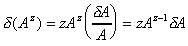
δ(Az) = zaz(δa/a)
In "sloppy" noatation, this is
δ(Az) = zAz(δA/A)
Remember that this result is an approximation, good only when the relative uncertainties are small.
Example
Let A = 5.23 <± 0.07. Evaluate F = A3.
First, the principle value is
P(F) = (5.23)3 = 143.056
Next applying our rule
| δ(F) | = zP(F)[δ(A)/P(A)] |
| = 3 × (5.23)3 × (0.07/5.23) | |
| = 5.744 |
So we have
F = 143.056 <± 5.744 .
Rounding down to one significant figure in the uncertainty yields
F = 143 <± 6 .
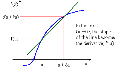
In terms of a formula, the definition of the derivative is
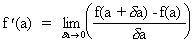 .
.
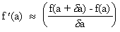
This can be rearranged to give,
f(a + δa) ≈ f(a) + δa × f ’(a)
Or if we had considered f(a-δa)
f(a - δa) ≈ f(a) - δa × f’(a)
And thus we have the general result that
f(a ± δa) ≈ f(a) ± δa × f’(a)
In our proper notation, A = a ± δa is the measurement. Then to first order
δ{f(A)} = δa × f ’(a)
Just to reiterate, this result is very good as long as δa is small compared to a, generally less than 10%. Some examples
|
|
|
|
|
|
|
|
|
|
|
|
|
|
|
|
|
|
|
|
|
|
|
|
|
|
|
|
|
|
|
|
|
|
|
|
WARNING: If you are dealing with trigonometric functions, δx must be in radians!
Examples
(i) Let θ = 1.23 <± 0.02 radians. Evaluate F = 3cos(θ).
First set your calculator to radians and determine the principle value
P(F) = 3cos(1.23) = 1.0027 .
Next, using the appropriate rule from the table above
| δ(F) | = 3δ(θ)sin(θ) |
| = 3 × 0.02 × sin(1.23) | |
| = 0.0565 |
Thus the answer is
F = 1.0027 <± 0.0565
We can only keep one figure in the uncertainty, thus
F = 1.00 <± 0.06
(ii) Let θ = 22.2 <± 0.2° . Evaluate F = ½tan(θ).
First set your calculator to degrees and determine the principle value
P(F) = ½tan(22.2°) = 0.2040 .
Next, using the appropriate rule from the table above
| δ(F) | = ½δ(θ)/[cos(θ)]2 |
| = ½ × (0.2° × π/180°)/[cos(22.2°)]2 | |
| = 0.0020 |
Thus the answer is
F = 0.2040 <± 0.0020
We can only keep one figure in the uncertainty, thus
F = 0.204 <± 0.002
Note that we have convert Δθ from degrees to radians in the error calculation.

This can be written as
δ{f(X)} = ½[f(x+δx) - f(x-δx)]
Example
Let A = 0.374 <± 0.009 . Evaluate F = arctan(A).
First set your calculator to radians or degrees and determine the principle value
P(F) = arctan(0.374) = 0.35789 rad = 20.506° .
The arctan function (labelled tan-1 on most calculators) is not in our table of functions, so we will use the quick approach.
First we evaluate the extremes
arctan(0.374 + 0.009) = 0.36577 rad = 20.957° ,
and
arctan(0.374 - 0.009) = 0.34997 rad = 20.052° .
Thus the uncertainty is
δ(F) = ½[0.36577 - 0.34997] = 0.0079 rad,
or
δ(F) = ½[20.957° - 20.052°] = 0.452° .
Hence we find F to be
F = 0.358 <± 0.008 rad = 20.5 <± 0.5° .
Where we have kept only one figure in the uncertainty.
F = (A/B + C/D)½ ,
where A, B, C, and D are measurements and thus have uncertainties. We want to find an expression for the uncertainty in F, δF, which depends only on P(A), P(B), P(C), P(D), δ(A), δ(B), δ(C), and δ(D). Such an expression could be used over and over, in a computer spreadsheet for instance, for many different values of A, B, C, and D.
If we were doing this for one set of values of A, B, C, and D on a calculator, we would do bits at at a time. We would set X = A/B and Y = C/D so that
F = (X + Y)½ .
Next we would set Z = X + Y so that
F = Z½ .
At this point we have something for which we do have a rule. We use the power rule to find that the uncertainty in F in terms of Z is
δ(F) = ½[P(Z)]-½δ(Z)
We know that the uncertainty in Z = X + Y is given by the addition rule, δ(Z) = [δ(X) + δ(Y)]. So we have
δ(F) = ½[P(Z)]-½[δ(X) + δ(Y)]
In turn, we use our division rule for calculating the uncertainties in X = A/B and Y = C/D. This yields δ(X) = P(A/B)[δ(A)/P(A) + δ(B)/P(B)] and δ(Y) = P(C/D)[δ(C)/P(C) + δ(D)/P(D)]. Hence
δ(F) = ½[P(Z)]-½[P(A/B){δ(A)/P(A) + δ(B)/P(B)} + P(C/D){δ(C)/P(C) + δ(D)/P(D)}]
Or more simply, this is
δ(F) = ½(f)-1[(a/b){δa/a + δb/b} + (c/d){δc/c + δd/d}] ,
where we have made use of the fact that f = P(Z)½.
The order of mathematical operations is functions, powers, multiplication or division, and then addition or subtraction. However when we write uncertainty expressions, we work from the outside in. This can be seen if we redo the operations above
| δ(F) | = δ{(A/B + C/D)½} | |
| = ½(a/b + c/d)-½δ{A/B + C/D} | power rule | |
| = ½(a/b + c/d)-½δ{A/B + C/D} | tidying up | |
| = ½(f)-1δ{A/B + C/D} | tidying up | |
| = ½(f)-1[δ{A/B} + δ{C/D}] | addition rule | |
| = ½(f)-1[(a/b)(δa/a + δb/b) + (c/d)(δc/c + δd/d)] | division rule |
In "sloppy" notation, this would be written
δF = ½(F)-1[(A/B)(δA/A + δB/B) + (C/D)(δC/C + δD/D)]
Examples
(i) Let A, B, and θ = φ±Δφ be measured quantities. Find an expression for δ(F) where F = A - Bcosθ.
The solution is
| δ(F) | = δ(A - Bcosθ) |
| = δ(A) + δ(Bcosθ) | |
| = δ(A) + P(Bcosθ)[δ(B)/P(B) + δ(cosθ)/ P(cosθ)] | |
| = δa + bcosφ[δb/b + (δφ × sinφ)/cosφ] |
In "sloppy" notation, this would be written
δF = δA + Bcosθ[δB/B + (Δθ × sinθ)/cosθ]
Note δφ must be in radians!
(ii) Let I, L, and R be measured quantities and μ0 be exact. Find an expression for the relative uncertainty in F = (μ0/2π)(I2L/R).
The absolute uncertainty is
| δ(F) | = (μ0/2π)δ{I2L/R} |
| = (μ0/2π)P(I2L/R) [δ(I2)/P(I2) + δ(L)/P(L) + δ(R)/P(R)] | |
| = P(F) [δ(I2)/P(I2) + δ(L)/P(L) + δ(R)/P(R)] | |
| = P(F) [{2P(I)δ(I)/P(I)}/P(I2) + δ(L)/P(L) + δ(R)/P(R)] | |
| = F [2δI/I2 + δI/I + δR/R] |
Note the use of the "sloppy" notation.
The relative uncertainty is δ(F)/P(F). Thus
δF/F = 2δI/I2 + δL/L + δR/R
(iii) Let M, G, and A be measured quantities. Find an expression for δ(X) where X = M(G-A).
| δ(X) | = δ{M(G-A)} |
| = P[M(G-A)][δ(M)/P(M) + δ(G-A)/P(G-A)] | |
| = P[M(G-A)][δ(M)/P(M) + {δ(G) + δ(A)}/P(G-A)] | |
| = M(G-A)[δM/M + (δG + δA)/(G-A)] | |
| = (G-A)δM + M(δG + δA) |
(iv) Let M, G, and A be measured quantities. Find an expression for δ(Y) where Y = MG - MA.
| δ(Y) | = δ(MG - MA) |
| = δ(MG) + δ(MG) | |
| = MG(δM/M + δG/G) + MA(δM/M + δA/A) | |
| = GδM + MδG + MδA + AδM | |
| = (G+A)δM + M(δG + δA) |
Notice in examples (iii) and (iv) that, although X = Y, we found that δX does not equal δY. Something funny is going on. Which is correct? To find out we would substitute M = m ± δm, G = g ± δg, and A = a ± δa into X or Y and find the maximum value of the uncertainty.
x ± δx = (m ± δm) [(g ± δg) - (a ± δa)]
Clearly, the biggest X can be is
x + δx = (m + δm) [(g + δg) - (a - δa)]
Keeping only first order terms, this becomes
x + δx = m(g-a) + m(δg + δa) + δm(g - a)
Thus the uncertainty in X is indeed
δX = (G-A)δM + M(δG + δA)
Why was δY incorrect? Let's look at the expansion
y ± δy = (m ± δm) (g ± δg) - (m ± δm)(a ± δa)
What is the biggest possible value of Y? You might suggest
y + δy = (m + δm) (g + δg) - (m - δm)(a - δa)
This is what we did in example (iv). Notice, however, that we have used two different values for M, m + δm and m - δm. This is not allowed. A variable can only have one value at a time.
The more complicated an expression is, the harder it is to determine the "correct" error formula. However, we need not be unduly concerned as we only keep one figure in the uncertainty and the difference between δX and δY should mainly be in the second figure if we are dealing with small uncertainties. As a rule of thumb, expressions involving subtraction should be factored, i.e. common variables taken outside a bracket, before the rules are applied.
| i) |  |
ii) | 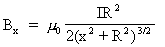 |
| iii) |  |
iv) | 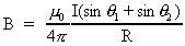 |
| v) | 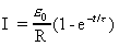 |
vi) |  |
| i) |  |
| ii) |  |
| iii) |  |
| iv) |  |
| v) |  |
| vi) |  |
Questions?mike.coombes@kpu.ca
![[Return to Kwantlen Homepage]](http://www.kpu.ca/images/return_button.gif)